Algebraic Curve Segments (Including Conic Segments)


The purpose of this report is to present a number of algebraically defined curve segments which have proven to be useful for representing the geometry of aerospace configurations and for the fitting of engineering data. The definitions that are shown for the various curve segments are some of the preliminary results of an effort to formulate algebraic analogies of French curves. These analogies will serve as the foundations of a curve fitting technique that is being developed for computer aided design applications. The curve segments that are presented here are both conic sections and conic like functions
The algebraic analog that is described here models, in a limited way, how a French curve can be used to smooth and interpolate points on a data curve.
Step 1: Select the appropriate French curve based on a visual inspection of the data plot.
Step 2: Positioning the French curve over that data plot to match the coordinates on the data plot.
Applying Algebraic Curve Segments follow the same steps.
Step 1: Select an equation whose graph has the same shape as the data plot.
Step 2: Evaluate the coefficients of the Curve Segment by matching the coordinate and slope conditions presented by the data plot.
The selection of an appropriate Curve Segment can be simplified by the use of a graphical dictionary displaying a collection of Curve Segments along with their equations and graphs.
The analytical curve segments are developed by first selecting the general form of the equation to be used for the curve fit and then determining the coefficients that are required to complete the definition of the curve fit.
The coefficients of the function are evaluated by satisfying boundary conditions as well as auxiliary conditions that the curve fit must satisfy. The standard boundary conditions that are to be considered are the end point locations and end point tangents. Typical auxiliary conditions could be the location and value of an internal extremum.
Experience has shown that the selection of the appropriate form for the curve fit is very straightforward and poses no more of a problem then the selection of the appropriate French curve.
The system of equations that determine the coefficients of the curve fit have been simplified by re-writing the general equation so that the graph of the Curve Segment will pass through the origin. This new equation will be referred to as the relative form of the general equation. The end points ( X1 , Y1 ) and ( X2 ,Y2 ) also shifted to the origin and become (0 , 0) and . The end point tangents T1 and T2 remain unchanged.

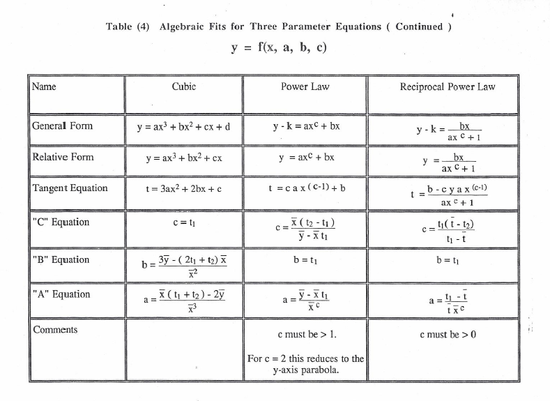
The system of equations that determine the coefficients of the algebraic curve segments are as follows: