Aitken’s Graphical Construction for a Parabola

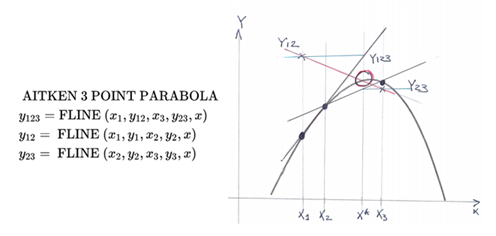
This paper presents a detailed demonstration of the exact nature of Aitken’s construction for generating points on a parabola.

It also introduces the FLINE, a function for generating points on a line, providing a direct way to encode Aitken’s construction.

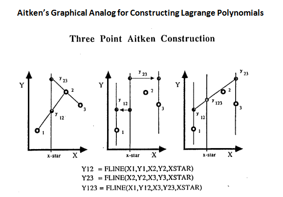
It will be shown that points on a parabola generated by Aitken’s construction are identical to the points generated by a second order Lagrange polynomial.

Additional work shows how to construct tangents on the Parabola.

Please note: MathPix, GreenShot, Notepad++ proved to be extremely helpful in composing this paper.

Aitken, A. (1932). On Interpolation by Iteration of Proportional Parts, without the Use of Differences. 

Proceedings of the Edinburgh Mathematical Society, 3(1), 56-76. doi:10.1017/S0013091500013808

Introducing FLINE to evaluate points on the line defined by end points (X1, Y1) and (X2, Y2),

it is then easy to encode Aitken’s Construction

Expanding and collecting like terms:

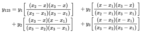
reproduces the second order Lagrange polynomial.

A Side note:

Generating a point using Lagrange polynomial requires 3 divisions, 15 multiplications, 6 subtractions and 3 additions.

On the other hand, Aitken formulation only requires 3 divisions, 6 multiplications, 9 subtractions and 3 additions.

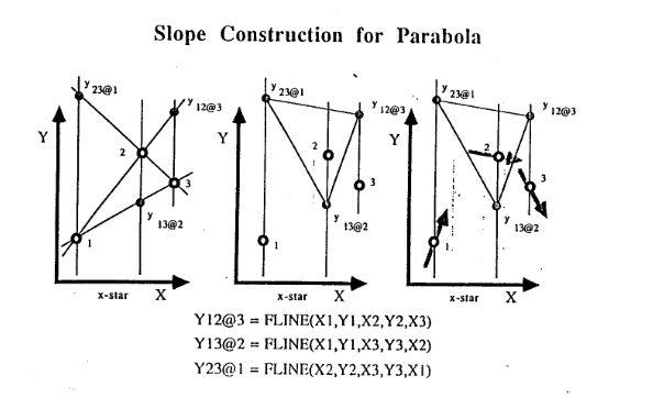
Extension of the Construction to Evaluate the Tangents at Defining Points of the Parabola

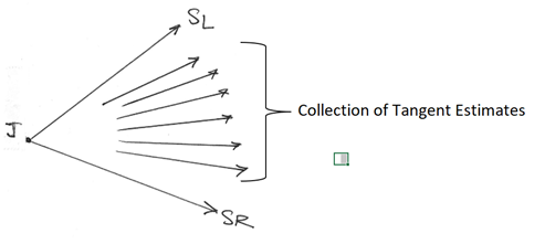
Using FLINE as a point of focus. Further examination of the Aitken Construction led to the realization that local tangents to the parabola could also be constructed.

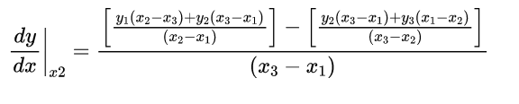
The development of the construction will begin with the polynomial. Taking the first derivative of Lagrange Polynomial

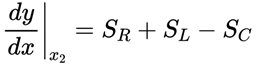
and evaluating it at a particular point say (X2, Y2)
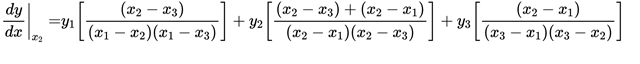
Continuing:

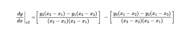
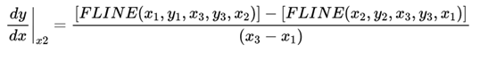
The Tangent at point (X2, Y2) can then be express in terms of FLINE

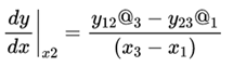
Continuing, all three tangents can then be evaluated

It should be noted that:

Showing how the tangent can be computed from the secants.

SLOPE: Numerical Differentiation of Tabular Functions

Introduction

This report presents a unique approach for the Numerical Differentiation of Tabular Functions. This approach focuses on the local shape of the Tabular Function, selecting all sets of three adjacent data points. The key features of this process are represented in the following diagrams.

Consider a typical interval of the Tabular function. Focus on point J, where the Data Point J runs from Point 2 to  Point N-1. At each interval construct, the Secants related to the adjacent points.

The Slope at Point J is estimated by the average of the Tangent Estimates that fall between the   MIN(SL, SR) and the MAX(SL, SR).

The notion of employing averaging as a means to stabilize the slope computation was inspired by various descriptions of Numerical Integration techniques that use sequential averaging to produce a smooth integral, suppressing irregularities in Tabular Functions.

Tangent Estimators

With the three points that make up each interval of the Tabular Function, it is possible to develop local fits to the data based on conic sections.

The complete formula for a conic curve is the classical formula:

Recognizing that the conic segment models must include the terms to support translation in both the X and Y directions (the slope of the curve is invariant under translation), gives rise to the choice of seven conic segments that can be defined by three points:

The detailed derivation of the central differences provided by the tangent estimators is given in a supporting document.

A Collection of Tangent Estimates for Numerical Differentiation.pdf

https://www.dropbox.com/s/bxzx98eli7qubrl/Aitken%20Graphical%20Constructions%20for%20Points%20on%20a%20Parabola.pdf?dl=0

Evaluating Tangent Estimators

The equations for all the Tangent Estimators are folded into a single subroutine. Computing numerators and denominators separately provide a simple control method to avoid the issue of division by zero.

Slope Estimates for the First and Last Data Points

The slopes of the first and last data points are computed using an extrapolation based on the Aitken construction for a Parabola.

Details of the Aitken Construction can be found here:

Aitken Graphical Constructions for Points on a Parabola.pdf

https://www.dropbox.com/s/bxzx98eli7qubrl/Aitken%20Graphical%20Constructions%20for%20Points%20on%20a%20Parabola.pdf?dl=0

Arc Length Calculation for 2-D and 3-D Tabular Functions

Arc Length Routines ARCLNG and ARCXYZ

My routines for estimating the arc length of a curve follow the concept of covering the curve with a collection of circular arcs. Examples of this concept can be found in Technical Drafting Text Books.

Following my focus of examining the local behavior of the curve by working with a sliding set of three points

Using a sliding set of three points to capture the local behavior of the curve presents then the image of a circumscribing circle for each set of three points.

Heron’s formula provides a direct way to compute the area a triangle with sides: a, b and c.

Letting s be the semi-perimeter of the triangle: s=(a+b+c)/2

Then the Area = SQRT(s(s-a)(s-b)(s-c))

This formula can be replaced with a simpler computation when the triangle is 2-D.

Area = 0.5 * ((xb – xa) * (yc – yb) + (xb – xc) * (yb – ya)) where the triangle vertices are:

(xa,ya) ,(xb,yb) and (xc,yc)

There are two important features to be noted about this process:

  1. The three points determine a plane as well as a circle.  Applying Heron’s formula for the Area allows this process to approximate the arc length of three-dimensional tabular functions.
  2. As the points slide along the curve, all interior intervals are covered by a left and right arc. My calculation averages the lengths of the two arcs.

ARCLNG – a subroutine to calculate the arc length of a two-dimensional curve.

The ARCLNG routine estimates the two-dimensional arc length distance starting from the first point to each point along the curve.

Usage:        CALL ARCLNG(X,Y,S)

Description of Parameters:

X          input vector of X-coordinate values (DIMENSION N)

Y          input vector of Y-coordinate values (DIMENSION N)

S          output vector of arc lengths (DIMENSION N)

ARCXYZ – a subroutine to calculate the arc length of a three-dimensional space curve.

The ARCXYZ routine estimates the three-dimensional arc length distance from the first point to each point along the curve.

Usage:        CALL ARCXYZ(X,Y,Z,S)

Description of Parameters:

X          input vector of X-coordinate values (DIMENSION N)

Y          input vector of Y-coordinate values (DIMENSION N)

Z          input vector of Z-coordinate values (DIMENSION N)

S          output vector of arc lengths (DIMENSION N)

Note:  The application of these routines is NOT limited to evenly spaced values of the argument.  However, abrupt changes in the spacing of the argument can have an adverse effect on the performance of this subroutine and should be avoided.   On the other hand, as with most numerical procedures, better results can be expected from uniformly spaced argument values.

It’s important to point out that these routines have incorporated two supporting routines that enable the efficient exchange of data between Excel worksheets and VBA arrays.

The way these are used:

Corrected Versions of the Workbooks for ARCLNG and ARCXYZ are available from DropBox

https://www.dropbox.com/l/scl/AABKirG-DWJMXDrLTOlbglZcD-ygq41TpBM

https://www.dropbox.com/l/scl/AACoSxLDbGgHtI1yIGVFD-q4sTl3aA0qin0

A User Controlled Demonstration of the Aitken-Lagrange Construction for Points on a Cubic.

Aitken Lagrange Cubic Construction

A few weeks ago Peter Bartholomew (uk.linkedin.com/in/peterbartholomew ) visited my blog. He made a very valuable suggestion – put up a demonstration for the construction of points on a cubic using the Aitken- Lagrange construction.
He sent me a sample workbook that demonstrated the point wise construction of a Bezier Cubic.
I have now re-engineered his workbook and have generated a user controlled demonstration for the Aitken-Lagrange construction of points on a cubic.
This workbook also demonstrates the technique of incorporating User Define Functions in Named Ranges. I believe that Bob Umlas (www.linkedin.com/pub/bob-umlas/46/278/479 ) was the first to discover this technique.
The User Defined Functions employed by this demonstration are:
Name Definition
X_Values =OFFSET(Aitken_Lagrange!$D1,0,0)

y_12_FLINE =(Y_P1*(X_P2-X_Values)+Y_P2*(X_Values-X_P1))/(X_P2-X_P1)
Y_23_FLINE =(Y_P2*(X_P3-X_Values)+Y_P3*(X_Values-X_P2))/(X_P3-X_P2)
Y_34_FLINE =(Y_P3*(X_P4-X_Values)+Y_P4*(X_Values-X_P3))/(X_P4-X_P3)

Y_123_FLINE =(y_12_FLINE*(X_P3-X_Values)+Y_23_FLINE*(X_Values-X_P1))/(X_P3-X_P1)
Y_234_FLINE =(Y_23_FLINE*(X_P4-X_Values)+Y_34_FLINE*(X_Values-X_P2))/(X_P4-X_P2)

Y_1234_FLINE =(Y_123_FLINE*(X_P4-X_Values)+Y_234_FLINE*(X_Values-X_P1))/(X_P4-X_P1)

Note well: The definition for the X_Values coming from Column D on Aitken_Lagrange Sheet enables the calculation of both the XStar lookup at the top of the sheet as well as the table of values at the bottom of the sheet.
The construction first evaluates Y_12_FLINE, Y_23_FLINE and Y_34_FLINE at XStar.
These results are the used to evaluate Y_123_FLINE and Y_234_FLINE at XStar.
And finally Y_1234_FLINE at XStar.

These steps can also be presented using the Functional Form for FLINE:
Function FLINE(ByRef XL As Double, _
ByRef YL As Double, _
ByRef XR As Double, _
ByRef YR As Double, _
ByRef XSTAR As Double) As Double
‘======================================
If Abs(XR – XL) > 0 Then
FLINE = (YL * (XR – XSTAR) + YR * (XSTAR – XL)) / (XR – XL)
Else
FLINE = 0.5 * (YL + YR)
End If
End Function

y_12_FLINE =FLINE(X_P1,Y_P1,X_P2,Y_P2,XStar)
Y_23_FLINE =FLINE(X_P2,Y_P2,X_P3,Y_P3,XStar)
Y_34_FLINE =FLINE(X_P3,Y_P3,X_P4,Y_P4,XStar)

Y_123_FLINE =FLINE(X_P1,Y_12_FLINE,X_P3,Y_23_FLINE,XStar)
Y_234_FLINE =FLINE(X_P2,Y_23_FLINE,X_P4,Y_34_FLINE,XStar)

Y_1234_FLINE =FLINE(X_P1,Y_123_FLINE,X_P4,Y_234_FLINE,XStar)

A User Controlled Demonstration of the Aitken-Lagrange Construction for Points on a Parabola.

Aitken Lagrange Parabola Construction

A few weeks ago Peter Bartholomew (uk.linkedin.com/in/peterbartholomew )visited my blog. He made a very valuable suggestion – put up a demonstration for the construction of points on a parabola using the Aitken- Lagrange construction.
He sent me a sample workbook that demonstrated the point wise construction of a Bezier Cubic.
I have now re-engineered his workbook and have generated a user controlled demonstration for the Aitken-Lagrange construction of points on a parabola.
This workbook also demonstrates the technique of incorporating User Define Functions in Named Ranges. I believe that Bob Umlas (www.linkedin.com/pub/bob-umlas/46/278/479 )was the first to discover this technique.
The User Defined Functions employed by this demonstration are:
Name Definition
X_Values =OFFSET(Aitken_Lagrange!$D1,0,0)

y_12_FLINE =(Y_P1*(X_P2-X_Values)+Y_P2*(X_Values-X_P1))/(X_P2-X_P1)
Y_23_FLINE =(Y_P2*(X_P3-X_Values)+Y_P3*(X_Values-X_P2))/(X_P3-X_P2)

Y_123_FLINE =(y_12_FLINE*(X_P3-X_Values)+Y_23_FLINE*(X_Values-X_P1))/(X_P3-X_P1)

Note well: The definition for the X_Values coming from Column D on Aitken_Lagrange Sheet enables the calculation of both the XStar lookup at the top of the sheet as well as the table of values at the bottom of the sheet.

My Tool Kit for Practical Numerical Tools for Tabular Functions

How the Toolkit came to be.

First realization 

  • I want my mathematics to be intuitive.
  • I want to see it.
  • I want to understand it.
  • I want to own it.

Second realization

  •  When applying curve fitting to physical data, knowing the theoretical behaviors does not make the error terms in the curve fit any smaller than if you did not know the theoretical behavior.
  • This then led me to focus the local behavior of a curve.
  • Focusing on three points at a time while sliding over the extent of the curve.

Third realization

  •  stacking the deck to facilitate the desired outcome is right and proper attitude for practical numerical techniques.

Fourth realization

  • Statement Functions in FORTRAN are cool.

The three seeds that formed the foundation of the Toolkit:

  1. A paper on Aitken’s Graphical Analog for Constructing Lagrange Polynomials
  2. A drafting textbook describing how a carpenter can measure arc length
  3. While reading textbooks on numerical analysis – there are always long glowing chapters on integration touting how averaging is the key to good results. While the very next chapter on differentiation is short and the author always advises the reader not to get involved. This led me to consider the possibility of incorporating an averaging technique into a process for numerical differentiation.