Foundation for the Numerical Analysis of Tabular functions

Foundation for the Numerical Analysis of Tabular functions

Typically engineering data is presented as a tabular function:

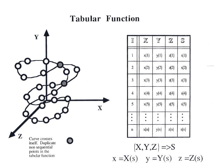
One way to analyze a tabular function is to develop an analytical function that approximates the data points of the tabular function and then operate on this function to calculate the required properties.

I have chosen an alternative approach that explores the local behavior of the tabular function focusing on a few data points at a time and then moving along the data points until the table has been completely explored.

Approximation of the arc length of a tabular function

My technique for calculating the arc length of a tabular function is a good example of this approach.

The details of the unit arc length:

There are two important features o be noted about this process:

1.  There are two circular arcs covering the interval between points 2 and point 3.

And since this is an empirical technique,   I choose to average the lengths of the left and right arcs.

2.       Three points also determine a plane and so with a slight adjustment to the calculation of the unit arc length this process can also be used to approximate three dimensional tabular functions.

The details of these two subroutines ARCLNG and ARCXYZ will be presented in detail along with a procedure for validating the reliability of this calculation.

Interpolation Based on Aitken’s Graphical Construction of Lagrange Polynomials

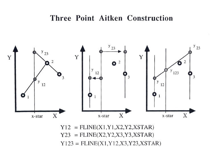
Continuing with this focus on three points at a time I have developed an interpolation technique based on Aitken’s graphical construction that replicated the use of Lagrange Polynomials.

I first saw a reference to this process in an article published in Design News an Engineering Trade Magazine. The paper presented a graphical construction attributed to Aitken that could generate additional points on a parabola defined by three points.

I was able to reduce the construction to a simpler form and with the use of my FORTRAN Statement function

FLINE(XL,YL,XR,YR,X) = (YL(XR-X)+YR(X-XL))/(XR-XL)

to replicate the construction with three calls to FLINE :

Y12=FLINE(X1,Y1,X2,Y2,XSTAR)

Y23=FLINE(X2,Y2,X3,Y3,XSTAR)

Y123=FLINE(X1,Y12,X3,Y23,XSTAR)

This technique is easily extended to produce the Lagrange cubic polynomial that is defined by four points:

While working with this construction I decided to make a modification.

Instead of forming

Y1234 = FLINE(X1,Y123,X4,Y234)

I formed

Y2233 = FLINE(X2,Y123,X3,Y234)

This modification produce a more pleasing fit for the interval between points 2 and 3 and so I was determined to discover the characteristics of the curve derived from the modified construction.

This effort led to two results:

1. The curve generated by the modified construction is a segment of a Hermetian Curve that passes through points 2 and 3. And is tangent to the Y123 Parabola at point 2 and tangent to the Y234 parabola at point 3.

2. The formulation of a construction for the tangent at each of the three points that define a parabola.

Slope at point 1 = (Y12@3-Y13@2)/(X3-X2)

Slope at point 2 = (Y12@3-Y23@1)/(X3-X1)

Slope at point 3 = (Y13@2-Y23@1)/(X2-X1)

For more information, contact me

alfred(dot)vachris(at)gmail(dot)com